- Publicado en
Fun with R
I've started to learn R using Coursera's Data Science Specialization and since I've completely forgot everything I knew about SciPy, I figured it would be a good idea to take some notes and make a post on some interesting things I've had to do so far.
So, the exercise is the following:
Say we have a set of log files for an application. Each entry from a log file has the following format:
HH:MM:SS Operation #n took X ms to complete.
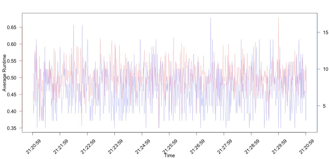
For each second, we want to find out the average and max time of operation #3 and create plot with this information. Also, we would like to see how many operations were running concurrently on each second using the same plot.
Creating the log files
To create the log files, we simply create a sequence of seconds and add some operations (between 1 and 16)
to each of them. Pro tip: Using cat to write the files is much faster than writeLines.
set.seed(20)

library(lubridate)

# now <- now()
now <- ymd_hms("2015-09-20 21:30:00")
logfiles <- c("logfile1.log", "logfile2.log")
for(output.file in logfiles){
  if(file.exists(output.file))
    file.remove(output.file)
  time.span = format(seq(now - minutes(10), now, by = "1 sec"), "%H:%M:%S")
  for(sec in time.span){
    cat(paste(sec, 'Operation # 3 took', rnorm(1,0.5,0.1), 'ms'), "\n", file = output.file, append = TRUE) # Make sure there is at least one operation of type 3 to avoid holes in the graph
    replicate(sample(1:15,1), cat(paste(sec, "Operation #", sample(1:3,1), 'took', rnorm(1,0.5,0.1), 'ms'), "\n", file = output.file, append = TRUE))
  }
}
Parsing the log files and obtaining the relevant information
Although these files are pretty clean when compared to what one would probably encounter on a real life situation, using grep, grepl or str_match can be enough for parsing them.
While writing this post I noticed that data.table is very picky with POSIXltdates, if you want to
have some fun, uncomment the next commented line.
library(stringr)
library(data.table)

time.pattern <- "(.*) Operation # 3 took (.*) ms"
data <- NULL
for(input.file in logfiles){
  con <- file(input.file)
  lines <- readLines(con)
  close(con)
  tmp.dt <- data.table(str_match(lines, time.pattern))
  setnames(tmp.dt, c("V1", "V2", "V3"), c("line", "date", "runtime"))
  data <- rbind(data, tmp.dt[!is.na(line)])
}
summary(data)
# data$date = hms(data$date) Don't do it. data.table is very picky with dates
data$runtime = as.numeric(data$runtime)
summary <- data[, list(avg.time = mean(runtime), max.time = max(runtime), n = .N), by = date]
Plotting
Now that the data is ready, it is only a matter of plotting it. I'm not going to use ggplot but the base R plotting functionality. In order to be able to add all information to the same plot disregarding whether this is a good or a bad practice, the plot must be created step by step. While doing this I found the max-time dots to create too much noise so the line where they are added is commented out.
xPoints <- seq_along(time.span)
plot(avg.time ~ xPoints, xlim = c(0,max(xPoints)), data = summary, type='l', ann = FALSE, col = '#FF000060', axes = FALSE)
axis(2, ylim = range(summary$avg.time), col = 'red', las = 1)
mtext(side = 2, line = 2.6, "Average Runtime")
mtext(side = 1, line = 3.5, "Time")
box()
## Let a second plot appear
par(new = TRUE)

#points(max.time ~ xPoints, data = summary, xlab = '', ylab = '', col = '#0000FF60')
plot(n.ops ~ xPoints, data = summary, type = 'l', ann = FALSE, col = '#0000FF60', axes = FALSE)
axis(4, at = pretty(range(summary$n.ops)), col = 'blue', las = 1)
mtext(side = 4, line = 2.5, "Number of Operations")

xLabels = seq(0, max(xPoints), 60)
axis(1, at = xLabels, labels = FALSE)
text(xLabels, time.span[xLabels], srt = 45, pos = 1, y = 0, xpd = TRUE)

Conclusion
R is very powerful, not a lot of code is necessary to do very interesting things with data. However, I find it very common to encounter small things that get in the way (data.table and plot, I'm looking at you ಠ_ಠ) and for which solutions are not evident.
The code used for this post can be found here